ContourPlot1

Contour Plots with a Color Gradient

Click to enlarge

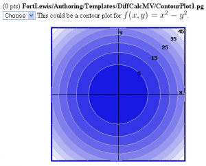
This PG code shows how to construct a contour plot with a color gradient.

• File location in OPL: FortLewis/Authoring/Templates/DiffCalcMV/ContourPlot1.pg

Templates by Subject Area

PG problem file	Explanation
Problem tagging data	Problem tagging:
DOCUMENT(); loadMacros( "PGstandard.pl", "MathObjects.pl", "PGgraphmacros.pl", "parserPopUp.pl", ); TEXT(beginproblem()); $refreshCachedImages = 1;	Initialization: We will use PGgraphmacros.pl for constructing the graph. Don't forget to have the browser cache refreshed by setting $refreshCachedImages = 1;
Context("Numeric")->variables->are(t=>"Real",x=>"Real",y=>"Real"); # # Create a graph canvas # $gr = init_graph(-5,-5,5,5,axes=>[0,0],pixels=>[300,300]); $gr->lb('reset'); $gr->lb( new Label(4.7,0.2,'x','black','center','middle')); $gr->lb( new Label(0.2,4.7,'y','black','center','middle')); # # A subroutine for adding the color gradient to the graph object # sub makegradient # ($graph, $steps, $r0, $g0, $b0, $r1, $g1, $b1) { my ($graph, $steps, $r0, $g0, $b0, $r1, $g1, $b1) = @_; my $dr = ($r1 - $r0) / $steps; my $dg = ($g1 - $g0) / $steps; my $db = ($b1 - $b0) / $steps; my $r = $r0; my $g = $g0; my $b = $b0; for my $i (0..$steps-1) { $graph->new_color("gradient$i",$r,$g,$b); $r += $dr; $g += $dg; $b += $db; } return $graph; } # # Add to $gr a 10 step color gradient # $gr = &makegradient($gr, 10, 0,0,225, # RGB blue 255,255,255 # RGB white ); # # Circular contours as parametrized curves # foreach my $k (5,10,15,20,25,30,35,40,45) { my $a = sqrt($k); $fn = new Fun( Formula("$a*cos(t)")->perlFunction, Formula("$a*sin(t)")->perlFunction, $gr ); $fn->domain(0,6.3); $fn->color("gray"); $fn->steps(60); $fn->weight(1); } # # Fill with gradient colors between contours # foreach my $i (0..9) { my $a = sqrt(2)/2 * sqrt(5*$i) - 0.1; $gr->fillRegion([ $a, $a, "gradient$i"]); $gr->fillRegion([-$a, $a, "gradient$i"]); $gr->fillRegion([-$a,-$a, "gradient$i"]); $gr->fillRegion([ $a,-$a, "gradient$i"]); } # # Label the contours # foreach my $k (5,15,25,35,45) { $gr->lb( new Label(0.707*sqrt($k),0.707*sqrt($k),$k,'black','center','middle')); } $pop = PopUp(["Choose","True","False"],"False");	Setup: By default, graph objects only know a few named colors, so if you want to have a color gradient, you'll need to add a bunch of named colors to the graph. The makegradient subroutine adds colors named gradient0, gradient1, ... to the graph object. Colors need to be specified in RGB format, and the makegradient subroutine takes in a graph object, the number of distinct colors you want in the gradient, a starting color (in this case blue) and an ending color (in this case white). Unfortunately, we have to do everything manually, including constructing the contour curves as parametric curves, filling the spaces between curves with colors from the color gradient, and labeling each contour curve.
Context()->texStrings; BEGIN_TEXT \{ $pop->menu() \} This could be a contour plot for \( f(x,y) = x^2 - y^2 \). $BR $BCENTER \{ image(insertGraph($gr),width=>300,height=>300,tex_size=>450) \} $ECENTER END_TEXT Context()->normalStrings;	Main Text: We ought to have asked a more interesting question.
$showPartialCorrectAnswers = 0; ANS( $pop->cmp() );	Answer Evaluation:
Context()->texStrings; BEGIN_SOLUTION Solution explanation goes here. END_SOLUTION Context()->normalStrings; COMMENT('MathObject version.'); ENDDOCUMENT();	Solution:

Templates by Subject Area