Difference between revisions of "Graph3DRectangular1"
Paultpearson (talk | contribs) m |
Paultpearson (talk | contribs) |
||
| Line 5: | Line 5: | ||
This PG code shows how to use the LiveGraphics3D Java applet to display an interactive graph of a function in rectangular coordinates. |
This PG code shows how to use the LiveGraphics3D Java applet to display an interactive graph of a function in rectangular coordinates. |
||
</p> |
</p> |
||
| − | * Download file: [[File:Graph3DRectangular1.txt]] (change the file extension from txt to pg when you save it) |
||
| + | * File location in OPL: [https://github.com/openwebwork/webwork-open-problem-library/tree/master/OpenProblemLibrary/FortLewis/Authoring/Templates/DiffCalcMV/Graph3DRectangular1 FortLewis/Authoring/Templates/DiffCalcMV/Graph3DRectangular1/Graph3DRectangular1.pg] |
||
| − | * File location in NPL: <code>FortLewis/Authoring/Templates/DiffCalcMV/Graph3DRectangular1/Graph3DRectangular1.pg</code> |
||
<br clear="all" /> |
<br clear="all" /> |
||
| Line 173: | Line 172: | ||
Context()->texStrings; |
Context()->texStrings; |
||
BEGIN_SOLUTION |
BEGIN_SOLUTION |
||
| − | ${PAR}SOLUTION:${PAR} |
||
Solution explanation goes here. |
Solution explanation goes here. |
||
END_SOLUTION |
END_SOLUTION |
||
Revision as of 17:23, 16 June 2013
Interactive Graph of a Function in Rectangular Coordinates in 3D
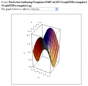
This PG code shows how to use the LiveGraphics3D Java applet to display an interactive graph of a function in rectangular coordinates.
- File location in OPL: FortLewis/Authoring/Templates/DiffCalcMV/Graph3DRectangular1/Graph3DRectangular1.pg
| PG problem file | Explanation |
|---|---|
|
Problem tagging: |
|
DOCUMENT(); loadMacros( "PGstandard.pl", "MathObjects.pl", "parserPopUp.pl", "LiveGraphicsRectangularPlot3D.pl", ); TEXT(beginproblem()); |
Initialization:
We need to include the macros file |
Context("Numeric");

Context()->variables->are(x=>"Real",y=>"Real",r=>"Real",s=>"Real",t=>"Real");

$a = - random(-1,1,2);

$plot = RectangularPlot3DRectangularDomain(
function => Formula("t^2+$a*s^2"),
xvar => "s",
yvar => "t",
xmin => -2,
xmax =>  2,
ymin => -2,
ymax =>  2,
xsamples => 10,
ysamples => 10,
axesframed => 1,
xaxislabel => "S",
yaxislabel => "T",
zaxislabel => "Z",
outputtype => 4,
);

if ( $a == -1) {
  $im = "hyperbolic-paraboloid.png";
  $pop = PopUp(
     ["Choose","Paraboloid","Hyperbolic paraboloid"],
     "Hyperbolic paraboloid");
} else {
  $im = "paraboloid.png";
  $pop = PopUp(
     ["Choose","Paraboloid","Hyperbolic paraboloid"],
     "Paraboloid");
}
|
Setup:
We generate a string of plot data using
Setting |
Context()->texStrings;
BEGIN_TEXT
The graph below is called a
\{ $pop->menu() \}
$PAR
$BCENTER
\{
Live3Ddata(
$plot,
image => $im,
size => [400,400],
tex_size => 600,
tex_center => 1,
scale => 1.1,
);
\}
$ECENTER
END_TEXT
Context()->normalStrings;
|
Main Text:
To display the string of plot data
After you construct the graph you like, don't forget to take a screen shot of it and make image files such as |
$showPartialCorrectAnswers = 1; ANS( $pop->cmp() ); |
Answer Evaluation: |
Context()->texStrings;
BEGIN_SOLUTION
Solution explanation goes here.
END_SOLUTION
Context()->normalStrings;

COMMENT('MathObject version.');

ENDDOCUMENT();
|
Solution: |
